In the example if the first grade is worth 60 and the second grade is worth 40 then type 60 in B2 and 40 in B3. Whenever we fill down the formula will always refer to the Weight row.

How To Calculate A Weighted Average In Excel

To calculate a weighted average in Excel simply use SUMPRODUCT and SUM.

How to calculate weighted grades excel. As we reach finals week were all thinking about December 15th and turning in final grades. Weighted mean has so many practical applications like calculating the average return of the portfolio calculating average grades in examinations finding the cost of capital in capital projects WACC finding the inventory value at end of the period when prices are changing etc. For the Number1 box select all of the weights.

Next navigate to the Formulas menu select the Math Trig drop-down scroll to the bottom and click on the SUM function. The Shortcut to Creating Weighted Grades Using Excel 2007. If you need the weighted average as well you would then apply this formula.

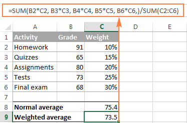
The last two columns of the first table display the normal average and the weighted average for a certain test quiz etc. To find the grade multiply the grade for each assignment against the weight and then add these totals all up. Giacomo Rambaldi Last modified by.

Use the RANK and PERCENTRANK functions in MS Excel. Not too long ago for most of us that meant sitting at a table with a calculator figuring out weights and averages. Make a gradebook based on percentage scores in Excel.

So for each cell in the Total column we will enter SUMGrade Cell Weight Cell so my first formula is SUM B2C2 the next one would be SUM B3C3 and so on. In this video SUMPRODUCT will basically multiply 75 by 01 35 by 01 etc and then add the product of those numbers. So basically weighted mean overcome the issues which simple.

The Function Arguments window will appear. Make an Excel gradebook that drops the 2 lowest scores. In Excel this can be represented with the generic formula below where weights and values are cell ranges.

6102006 73923 AM Other titles. AVERAGE D5D7 with the range being the score for that subject. To get the normal average you would use the following formula.

Exercise 1 - Weighted Scoring Sheet Excel Author. We can calculate a weighted average by multiplying the values to average by corresponding weights then dividing the sum of results by the sum of weights. Calculate weighted.

Select the cell where you want the results to appear in our example thats cell D14. As mentioned earlier when computing for the weighted average youll have to multiply the values to their weights and add the products. Suppose your teacher says The test counts twice as much as the quiz and the final exam counts three times as much as the quiz.

Make an Excel gradebook that removes the lowest score. Type your grades in column A. In the example if the first grade is worth 60 and the second grade is.

In this case it will be 753535etc. Then instead of dividing the result with the total number of values youll have to divide the product of the first half of the formula with the sum of all the. Type the weight each grade has in column B next to its corresponding grade.

For example if you received a 95 and an 80 then type 95 in A2 and 80 in A3. Type the weight each grade has in column B next to its corresponding grade. 9101 65015 8002 73025 6803 010150202503735.

Type A2B2 in cell C2. SUMPRODUCTweights values. Was this step helpful.

First the AVERAGE function below calculates the normal average of three scores. In this example in order to calculate the weighted average overall grade you multiply each grade by the corresponding percentage converted to a decimal add up the 5 products together and divide that number by the sum of 5 weights. Below you can find the corresponding weights of the scores.

Weighted Grade Calculator Excel Template Source.